Through our previous article, we successfully created a dataset that combines movie snapshots and their respective tags describing what the image contains.
As a reminder, the dataset consists of 243 558 images with 183 different labels. It is a simple CSV file that looks like this:
| id | shot_image_id | tags |
|---|---|---|
| 1 | 1 | statue |
| 2 | 81091 | bed, legs, text |
| 7 | 250992 | hand, text |
| 8 | 81360 | castle, sky |
| 10 | 9 | water, redhead |
Our final dataset: an image ID and its tags.
We are now going to use this dataset to create and train an AI that will be able to detect and suggest elements of the images uploaded by users. But how to do that? What library can we pick to make this AI? Where are we going to find the CPU and GPU ressources needed to train our AI quickly?
In this second part of the series, we are first going to find and create an environment suitable for this heavy task. Then, we will pick FastAI, one of the most promising deep learning librairies available nowadays, to make our AI and hopefully have, at the end of the article, a good model that we could export in order to use it on our website.
# Set-up the environment
To train our AI with FastAI, we need to find the best environment available that can handle working over 250 000 images in a short time. Our website runs on two dedicated servers with great hardware to serve a Ruby on Rails app. But Computer Vision needs a lot of ressources, especially a good GPU — which our servers don’t have. Therefore, we need to find a platform that can give us these ressources for a cheap price or even for free, on demand.
That’s fortunate since there are two main platforms online which can provide in a very easy way the environment we are looking for.
# Kaggle, a place for data science projects
Kaggle is a well-known community website for data scientists to compete in deep learning challenges. After joining a competition, you are given a dataset and you have to create an AI that gives the best results on it. You are free to use any deep learning library you wish to.
But say that Kaggle is only about competitions would be incorrect. In fact, Kaggle also provides to data scientists hundreds of datasets for free to work on, courses to learn the most used tools in the field and more importantly, a ready-to-use environment with great ressources for free.
You can then join competitions and fight with other data scientists directly on their website. They give you everything you need: a Jupyter-like interface, some disk space, a good CPU and a GPU. Within a few clicks, you can start training an AI!
FastAI, the library we are about to use for this project, is available on Kaggle as well. Actually, this project was heavily inspired by this kernel that you can fork where Jeremy Howard — the creator of FastAI — , use his library to participate to the famous Planet: Understanding the Amazon from Space competition. He got excellent results with only a few lines of code.
You can find a nice tutorial on how to start using FastAI on Kaggle on their official website.
While Kaggle seems to be the perfect place for our project, it has some limitations. I see Kaggle as a nice website where you can play and try different kind of things. But for serious deep learning projects, you will have to switch to a real provider that gives you more flexibility, more ressources.
# Google Cloud Platform
Since we want to be able to export our model and re-train our AI every month in an automatic way, we need to find a better host for our task where we can deeply custom our environment according to our needs. Google Cloud Platform seems to be the perfect place for that matter. It provides many services for a reasonable price. You can even get 300$ of credits for free for one year when registering.
Working with GCP definitely requires more time and more work. You basically have to create a Virtual Machine and install everything you need for your project. The main advantage though is that you are free to create any kind of Virtual Machines for your project. You can set-up a VM with large ressources and even pick the region across the world where the VM would be located.
Fortunately, there are plenty of tutorials available online to get you started on GCP. FastAI has a dedicated tutorial on how to start using their library on the Google Cloud Platform. After following their instructions, you should have an environment with all the tools necessary to start training an AI.
Having our environment on the cloud will definitely make things easier when we would have to re-train our model on monthly basis. GCP provides APIs for almost every service they offer including creating, starting and stopping VMs. That’s a really important feature that will make the re-training less difficult.
# Create an AI with FastAI
We created a VM running on Google Cloud Platform with a great GPU — a NVIDIA Tesla P100 with 16 gigabytes of VRAM in our case. Just like in our previous article where we created our dataset with Pandas, we are going to use Jupyter to interact with FastAI. But first, let’s talk about this awesome library.
The FastAI library offers a high-level API capable of creating deep learning models for a lot of different applications including text generation, text analysis, image classification and image segmentation. FastAI is for Pytorch what Keras is for Tensorflow: a more intuitive set of abstractions that make it easy to develop deep learning models in a few lines of code.
FastAI takes care of a lot of parameters or hyper-parameters for you and it results in good performance by default — everything is customizable of course.
But FastAI is not only a library, it is also a great course to get into deep learning. The course is splitted into two parts and is available on their website for free. It’s perfect for newcomers as it will let you play quickly with deep learning models without a huge knowledge of the field. This project is entirely based on this course and on FastAI so thanks to them for their awesome work!
Now let’s start coding! As usual, we first have to import all the librairies we need through Jupyter:
import pandas as pd
import numpy as np
import matplotlib.pyplot as plt
from fastai.vision import *

# see matplotlib charts on Jupyter
%reload_ext autoreload
%autoreload 2
%matplotlib inline
# Pre-processing the dataset
The first thing we would have to do is pre-processing our dataset. Pre-processing is a very important step, especially when dealing with images. To get better performance or even to let the neural network understand what we are feeding him, we have to normalize the images and resize them.
In our project, we are dealing with snapshots that come from movies. Movies can have many different aspect ratios. Think about old movies: most of them were made using a square format — 4/3. But nowadays, it’s all about widescreens — 16/9 — or even wider aspect ratios such as 2.35 or 2.39.
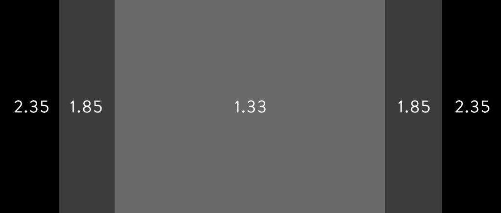 The most-used aspect ratios in the cinema industry.
Therefore, to make our AI more efficient, the pre-processing step is crucial: we need to make sure all our datas will have the same format for the training part. To do that, let’s first load our CSV file that contains our dataset:
path = Path('.')
data = ImageList.from_csv(path,
                          'dataset.csv',
                          cols=1, folder='images',
                          suffix='.jpg')
With these two lines of code, FastAI basically reads our dataset file and understands that our images are stored in a folder named “images” with the suffix .jpg. ImageList is a built-in function that lets you do computer vision easily. You can find more informations about this function or about the whole library on their great documentation section.
The variable data now contains everything related to our dataset. We can start the pre-processing:
data = data.split_by_rand_pct(0.1) # use 10% of our dataset as validation set
           .label_from_df(cols=2, label_delim=',') # get the tags
           .transform(get_transforms(), size=224, resize_method=3) # resize
           .databunch(bs=64) # use mini-batches of size 64
           .normalize(imagenet_stats) # normalize using the famous imagenet
Most of the comments speak for themselves but I will detail a little bit. The first thing we are doing is use the split_by_rand_pct method to split the dataset into two parts:
-
A training set: It will contain images and tags that will be used to train our AI. We take 90% of the original dataset for the training set.
-
A validation set: Images and tags that the AI is not using to learn. These images are only seen by the model to validate if it’s learning correctly and the performance is getting better or not. We use 10% of the original dataset for that matter — hence the value “0.1”.
Secondly, we are telling FastAI where to look for the labels of each image with the label_from_df method. In our case, the labels are located in the second column of our CSV file — not counting the index column — , and are delimited by a comma.
Then comes the interesting part, the pre-processing. With the transform method — and more specifically the get_transforms() function — , we are asking FastAI to perform some work on our images in order to create “more” data. This is called Data Augmentation. This is particularly useful when you don’t have enough datas in your training set. FastAI will apply by default some techniques to the training images at its disposal, the most common ones being affine transformations — like horizontal or vertical flip, rotation etc.
There are also non-affine transformations such as resizing, cropping, brightness variations and more. It will create on each iteration new variant of images based on a single one.

The next transformation we are doing is the resizing of the images which as you saw, is important in our case. We decided to pick the square size of 224 pixels by 224 pixels because it seems to be a good value for computer vision, especially when normalizing the image with ImageNet which we do on the last line.
We decided to pick the resize_method number “3”. It equals to the “squish” method. The other methods available were “crop”, “pad”, or no resizing at all.
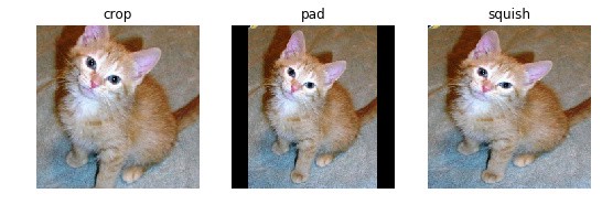 The difference methods available to resize our images.
We have chosen the “squish” method because after a few tests, we found out that it was the most suitable method in our case considering we wanted to keep all the informations of the original images after the resizing no matter their original size and aspect ratio. It gave us the best results every time.
Finally, we normalize our images using the ImageNet statistics. Normalization involves using the mean and the standard deviation of the famous ImageNet dataset. Using the mean and the standard deviation is a pretty standard practice. Since they are calculated using a million of images, the statistics are pretty stable. It will make the training faster.
# Define our neural network structure
Once we are done with the pre-processing, it is time to create the architecture of our neural network and start training our AI. We are going to use Transfer Learning for this project. Transfer learning is a technique where a model trained on one task is re-used on a second related task — in our case, detecting elements in movie snapshots. This kind of techniques can be very useful to help, for example, people that don’t have the knowledge to create from scratch their deep neural network neither the ressources or time. Or simply to avoid recoding something entirely when we can use a similar model that works nicely for our type of datas, out of the box.
We are going to use one of the most interesting models created recently for image classification called “Resnet” — the other models available are listed on Pytorch’s website. Resnet is a residual neural network available in several versions with a depth up to 152 layers — “Resnet152”. It offers incredible results in image recognition.
With transfer learning, we are going to take the pre-trained weights of this already trained model — that has been trained on millions of images belonging to 1000 different classes — and use these already learned features to predict new classes — our tags. The main advantage by doing so is that we don’t need an extremely large training dataset to get good results fast.
Let’s make our architecture with “Resnet152” as a pre-trained model and create a convolutional neural network which is widely used in computer vision. CNN is a Deep Learning algorithm which can take an image as input, assign importance to various aspects or objects in the image and be able to differentiate one from the other. Perfect for us!
acc_02 = partial(accuracy_thresh, thresh=0.2)
f_score = partial(fbeta, thresh=0.2)
learn = cnn_learner(data, models.resnet152, metrics=[acc_02,f_score])
We defined two functions that will be the metrics of our neural network to help us evaluate if it performs well. The first one is the accuracy threshold. Why a threshold? Simply because here, we are not making a multi-class classifier where we want our AI to predict only one class for every image — the one with the highest probability. We are making a multi-label classifier which means that every image can have different classes — or zero.
In our case, we have 183 different classes. So we are going to have one probability for each class for every image. But then, we are not just going to pick out only one of those, we are going to pick out n of those 183 classes. Basically, we compare each probability to some threshold. Then we are going to say that anything that is higher than this threshold means that the image does have that element in it. Jeremy Howard used 0.2 as a threshold for his competition as it seems to generally work pretty well1. We decided to follow his advices. Therefore, every class for a given image that have a probability higher than 0.2 will then be considered as part of the image.
The second metric is called “FBeta”. It is a well-known metric widely-used in the data scientists industry or in competitions hosted by Kaggle. When you have a classifier, you are going to have some false positives and some false negatives. How do you weigh up those two things to create a single number and evaluate the performance? There are a lots of different ways of doing that and the “FBeta” is a nice way of combining that into a single number. It takes in consideration the precision and the recall. You can read more about the “FBeta” on Wikipedia.
# Let’s start training
We have now a ready-to-use convolutional neural network with Transfer Learning, Resnet152 and two metrics. It’s time to train our data! Let’s start with 10 epochs — one epoch means an iteration over all our images.
learn.fit_one_cycle(10)
| epoch | train_loss | valid_loss | accuracy_thresh | fbeta | time |
|---|---|---|---|---|---|
| 0 | 0.028299 | 0.025567 | 0.992606 | 0.487419 | 32:35 |
| 1 | 0.026299 | 0.023810 | 0.992710 | 0.529195 | 32:45 |
| 2 | 0.025215 | 0.023037 | 0.992652 | 0.553807 | 32:58 |
| 3 | 0.024489 | 0.022692 | 0.992956 | 0.553749 | 33:15 |
| 4 | 0.023871 | 0.022190 | 0.992828 | 0.570699 | 33:06 |
| 5 | 0.023519 | 0.021935 | 0.992900 | 0.574040 | 32:58 |
| 6 | 0.023003 | 0.021534 | 0.992551 | 0.589838 | 33:06 |
| 7 | 0.023071 | 0.021359 | 0.992833 | 0.590645 | 32:57 |
| 8 | 0.022750 | 0.021231 | 0.992876 | 0.593163 | 32:46 |
| 9 | 0.022044 | 0.021225 | 0.992887 | 0.594099 | 32:53 |
Without that much of work, we get pretty good results already!
The accuracy seems fine and the FBeta keeps going up. The Fbeta score might seem low for some of you but remember that we are working over 183 different classes and we are not trying to make a perfect AI that could predict absolutely every element that an image contains. We are trying to make an AI capable of suggesting the most common tags used on the website such as “black and white”, “animation”, “man”, “woman” etc.
Still, there is place for improvements. We can try to adjust the learning rate of our neural network to see if it can lead to better results. The learning rate is a very important hyper-parameter in deep learning. If it is chosen poorly, the neural network won’t perform well. FastAI, by default, uses an one-cycle policy which means the learning rate will first increase over each iteration and then decrease.
The one-cycle policy allows to train a neural network very quickly, meaning it will converge fast to a low loss value. But to make it work, we need to find the optimum learning rate that will make the one-cycle policy really shine. FastAI provides functions to find the best learning rate:
learn.unfreeze()
learn.lr_find()
learn.recorder.plot(suggestion=True)

We can see on the chart above that a large learning rate doesn’t seem to help. In fact, the bigger the learning rate is, the bigger the loss is. And we don’t want that. We can restrain our learning rate to avoid this and start again the training with this updated parameter. Also, we are not only going to restart the training with only the last layers of our neural network being updated. Instead, we are going to update this time all the weights, including the Resnet’s 152 layers weights with the function unfreeze() used above.
learn.fit_one_cycle(10, max_lr=slice(1e-06,1e-04))
| epoch | train_loss | valid_loss | accuracy_thresh | fbeta | time |
|---|---|---|---|---|---|
| 0 | 0.022467 | 0.021131 | 0.992844 | 0.596691 | 42:52 |
| 1 | 0.022203 | 0.021018 | 0.992805 | 0.601539 | 40:42 |
| 2 | 0.021539 | 0.020817 | 0.992989 | 0.602677 | 40:57 |
| 3 | 0.021007 | 0.020594 | 0.992868 | 0.612011 | 42:45 |
| 4 | 0.020509 | 0.020398 | 0.992928 | 0.616314 | 40:44 |
| 5 | 0.019788 | 0.020305 | 0.992734 | 0.625013 | 40:57 |
| 6 | 0.018687 | 0.020285 | 0.993009 | 0.622852 | 42:56 |
| 7 | 0.018598 | 0.020303 | 0.992985 | 0.628156 | 40:44 |
| 8 | 0.018053 | 0.020240 | 0.992838 | 0.628797 | 40:59 |
| 9 | 0.018110 | 0.020274 | 0.992997 | 0.627074 | 42:42 |
The train loss seems to get lower and the FBeta seems to get higher as well. Everything looks awesome! We could try another learning rate and train a little more hoping to increase the performance of our model but we can see already that we are most likely in the optimal capacity that falls between underfitting and overfitting.
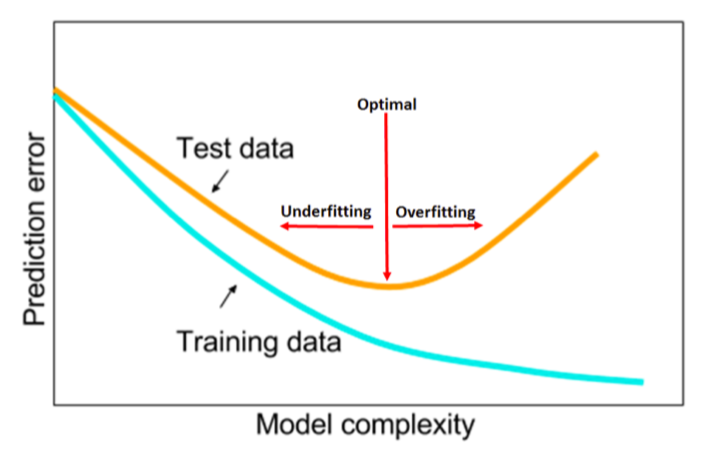
Indeed, after the 4th epoch, our validation loss starts to be higher than the training loss. But more importantly, it doesn’t seem to decrease anymore while in the meantime, the training loss keeps decreasing. We can even see that the validation loss starts to increase on some epoch. This is definitely a sign that we might have reached the optimal capacity of our model and we should stop the training here otherwise we might start overfitting.
Overfitting happens when you train too much your model on the same data. When it’s time to test your model on datas it has never seen, out of its comfort zone, the model starts to perform poorly because it only got used to recognize the training datas and nothing else. It does not generalize well on new, unseen data. The model learned patterns specific to the training data, which are irrelevant in other data.
# Predictions on test images
It’s better for us to stop the training here and call it a day. We can first save our model with the save() function and export our model with all the optimized weights and bias:
learn.save('res152-movie-stills-after-lr')
learn.export('movie-stills-tags-ai.pkl')
We can quickly test on a various number of images if our AI performs correctly on suggesting tags for movie snapshots. We put a hundred of movie stills the AI has never seen in a folder and created a quick Python script to show the predicted tags for each image with their respective probability:
import os

# load our pre-trained model we just exported
rest = load_learner(path, 'movie-stills-tags-ai.pkl')

for filename in os.listdir(path/'test'):
  img = open_image('test/' + filename)
  # resize the images the same way a the pre-processing
  img = img.apply_tfms(tfms=get_transforms()[1], size=224, resize_method=3)
  # get preds for each class and show only the one > to our thres
  preds, idx, output = rest.predict(img)
  d = dict({rest.data.classes[i]: round(to_np(p)*100,2) for i, p in enumerate(output) if p > 0.2})
  img.show(title=str(d))
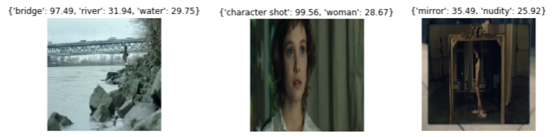
It seems to work well! Sure it does not list all the possible elements displayed in the image but that was never our goal. We wanted to create an AI that could suggest common tags to users when they upload movie snapshots and I think it works nicely. Almost two thirds of the time, the AI suggests all possible elements of the image. It doesn’t mean that the rest of the time it doesn’t suggest anything, just not all elements — maybe one or two tags only.
As always, there is room for improvement but for a first model, we are happy with the results. It’s important to remember that only tags that have more than 20% of probability of being present according to our AI are displayed here. We want to suggest tags that we are confident there really are inside the image.
# What’s next?
Now that we have done an AI capable of detecting elements in movie snapshots and exported the model with good performance after testing it briefly, how are we going to turn this single file into a service on our website? How are we going to implement the AI on our servers and interact with the current Ruby on Rails backend? That will be the theme of our next article where we will create a REST API in Python with Docker to allow our website to send requests to the AI which will return what tags are present in a given image. Stay tuned!
-
In the third video of his 2019 course, Jeremy Howard explains what a threshold is and why he picked 0.2. ↩
-
A disciplined approach to neural network hyper-parameters: Part 1 – learning rate, batch size, momentum, and weight decay. ↩